This practical work focuses on Pinehole Camera Calibration using OpenCV and Python.
1. Preparation
The first dependency that is needed is OpenCV library that can be installed with the command:
pip install opencv-python
or for conda installation:
conda install -c conda-forge opencv-python
The second dependency is the MatPlotLib library that can be installed with the command:
pip install matplotlib
or for conda installation:
conda install -c conda-forge matplotlib
The MatPlotLib library displays geometric rendering in an independent interactive window. Depending on the Python environment, this window may be rendered as a frozen image,
preventing user interaction. To correct this problem, here are a few solutions:
Jupyter Notebook:
Execute following code within the Jupyter Notebook: %matplotlib qt
PyCharm:
Go to Settings / Tool / Python Plot and uncheck the option Show plots in tool windows.
Spyder:
Go to Tools / Preferences / IPython console / Graphics / Backend:Inline and change "Inline" to "Automatic".
Click OK button and restart the IDE
2. Using OpenCV and MatPlot within Python program
OpenCV python binding relies on Numpy for the vector and matrix representation and on MatPlotLib for display. Using OpenCV within a Python program needs to import the three libraries:
import numpy as np
import cv2 as cv
import matplotlib.pyplot as plt
All Python program that uses OpenCV has to contain these imports.
|
Exercise 1. Create a python file calibration_chessboard.py that contains the following program: Run the program to ensure that all the dependencies are installed. |
3. Camera calibration
The pinhole camera model enables to describe the projection of a 3D point $P_{c}\ =\ (x_{c},\ y_{c},\ z_{c})$ onto an image $i$ as a 2D point $(u_{c}^{i},\ v_{c}^{i})$. More formally:
$$\left[{}\begin{array}{c}u_{c}^{i} \\ v_{c}^{i} \\ 1 \end{array}\right]{}\ =\ \left[{}\begin{array}{c} f_{u} & 0 & c_{u} \\ 0 & f_{v} & c_{v} \\ 0 & 0 & 1 \end{array}\right]\ \Delta{}\left({}\left[{}\begin{array}{c} \dfrac{r_{11}^{i}x_{c}\ +\ r_{12}^{i}y_{c}\ +\ r_{13}^{i}z_{c}\ +\ t_{x}^{i}}{r_{31}^{i}x_{c}\ +\ r_{32}^{i}y_{c}\ +\ r_{33}z_{c}\ +\ t_{z}^{i}} \\ \\ \dfrac{r_{21}^{i}x_{c}\ +\ r_{22}^{i}y_{c}\ +\ r_{23}^{i}z_{c}\ +\ t_{x}^{i}}{r_{31}^{i}x_{c}\ +\ r_{32}^{i}y_{c}\ +\ r_{33}z_{c}\ +\ t_{z}^{i}} \\ \\ 1 \end{array}\right]{}\right)$$
where $\Delta{}$ is the distortion computation:
$$\Delta{}\left({} \left[ \begin{array}{c} x_{p} \\ y_{p} \\ \alpha{} \end{array}\right]{}\right){}\ =\ \left[ \begin{array}{c} x_{p} \dfrac{1 + k_1 r^2 + k_2 r^4 + k_3 r^6}{1 + k_4 r^2 + k_5 r^4 + k_6 r^6} + 2 p_1 x_{p} y_{p} + p_2(r^2 + 2 x_{p}^2) + s_1 r^2 + s_2 r^4 \\ \\ y_{p} \dfrac{1 + k_1 r^2 + k_2 r^4 + k_3 r^6}{1 + k_4 r^2 + k_5 r^4 + k_6 r^6} + p_1 (r^2 + 2 y'^2) + 2 p_2 x_{p} y_{p} + s_3 r^2 + s_4 r^4 \\ \\ \alpha{} \end{array}\right],\ r\ =\ x_{p}^{2}+y_{p}^{2}$$
with:
- $f_{u}$, $f_{v}$ respectively are the horizontal and vertical focal lengthes, expressed in pixels
- $c_{u}$, $c_{v}$ are the coordinates of the principal point, expressed in pixels, within the image referential
- $k_{1}$, $k_{2}$, $k_{3}$ are the radial distortion coefficients
- $k_{4}$, $k_{5}$, $k_{6}$ are the radial distortion rational coefficients
- $p_{1}$, $p_{2}$ are the tangential distortion coefficients
- $s_{1}$, $s_{2}$, $s_{3}$, $s_{4}$ are the thin prism distortion coefficients
- $(x_{c},\ y_{c},\ z_{c})$ are the coordinates of the reference point $c$ (i-e the 3D coordinates of the corner $c$)
- $(u_{c}^{i},\ v_{c}^{i})$ are the coordinates of the projection of the reference point $c$ onto the image $i$
- The image $i$ pose is defined such as: $$\left[{} \begin{array}{c} r_{11}^{i} & r_{12}^{i} & r_{13}^{i} & t_{x}^{i} \\ r_{21}^{i} & r_{22}^{i} & r_{23}^{i} & t_{y}^{i} \\ r_{31}^{i} & r_{32}^{i} & r_{33}^{i} & t_{z}^{i} \\ 0 & 0 & 0 & 1 \end{array} \right]$$
This computation shows that some of the parameters are the same for all the projection equations that are coming from a same camera:
- $f_{u}$, $f_{v}$, $c_{u}$, $c_{v}$
- The distortion parameters $k$, $p$ and $s$
Determining these parameters enable to simplify the projection computation. The process that compute their values is called camera calibration.
3.1. Preparation
The first steps before calibrating a camera are to ensure that all the needed dependencies are set up and that it is possible to load images from files.
|
Exercise 2. Create a folder named data in the same directory as calibration_chessboard.py and download the images dataset from http://www.seinturier.fr/teaching/computer_vision/data/calibration-google_pixel_6.zip. Unzip the calibration-google_pixel_6.zip file within the data directory. Now the directory structure should be data/google_pixel_6/chessboard/6x11 and should contains images. Modify the calibration_chessboard.py program as follows: Run the program and ensure that are the images within data/google_pixel_6/chessboard/6x11 directory are listed. Expected result: Image list: Tip: The last file separator / may be a \ on window systems. |
The first step of the calibration process is the detection of references points (the corners of the chessboard). The detection algorithm works with gray images so dealing with calibration process needs to first load images with their color and then, convert them into grayscale. The loading and convertion of images with OpenCV is performed with the instructions:
img = cv.imread(image_file)

gray = cv.cvtColor(img, cv.COLOR_BGR2GRAY)
The first line load an image within OpenCV format, the second line convert the images to grayscale.
After a successful load, images can be displayed within MatPlotLib (the library can handle OpenCV images) using the instruction:
plt.figure(image_file)
plt.imshow(img)
plt.show()
The first line create a windows named according to the image_file we want to display. The second and thirs lines are displaying the image within the created windows. Please note that if various images have to be displayed, the last line plt.show() has to be called only once at the end:
plt.figure(name1)
plt.imshow(img1)
...
plt.figure(nameN)
plt.imshow(imgN)

plt.show()|
Exercise 3. Modify the calibration_chessboard.py program as follows: Ensure that when running the program, images are showing within MatPlotLib window. |
3.2. Chessboard configuration
Camera calibration process aims at optimizing a set of reference points with known 3D coordinates with their 2D projections on the image. It is common to use chessboard as reference points set. A chessboard is made of corners that can be organized in rows and columns:
 Each corner of the chessboard is a reference point with a known 3D coordinate. The reference points are listed from the chessboard top left to the chessboard bottom right (ie row by row from the top and column by column from the left). The coordinates of the reference point i are:
$$\left( \begin{array}{c}x_{i} \\ y_{i}\\ z_{i}\end{array} \right)\ =\ \left( \begin{array}{c}size\times{}((i-1)\ \text{div}\ cols) \\ size\times{}((i-1)\ \text{mod}\ cols) \\ 0 \end{array} \right)$$
where:
- $rows$ and $cols$ are the number of rows and the number of columns of the chessboard respectively
- $i$ is the index of the reference point, $1\leq{}\ i\ \leq{}rows\times{}cols$
- $size$ is the length of a square
The previous calculus can also be written:
$$\left( \begin{array}{c}x_{r\times{}cols+c} \\ y_{r\times{}cols+c}\\ z_{r\times{}cols+c}\end{array} \right)\ =\ \left( \begin{array}{c}r\times{}size \\ c\times{}size) \\ 0 \end{array} \right),\ \text{where}\ (r, c)\text{ are the row and the column of the corner}$$
|
Exercise 4. Modify the program calibration_chessboard.py in order to integrate chessboard characteristics. The function calibrate_chessboard(image_files) has now to start as follows: Run the program to check the reference points. Expected output: Reference points: [[ 0. 0. 0.] |
3.3. Chessboard detection
Performing calibration relies on finding the reference points (chessboard corners) projections on all images. OpenCV provide a function that enable to detect corners of a chessboard:
ret, corners = cv.findChessboardCorners(image, patternSize, corners, flags)The function attempts to determine whether the input image is a view of a chessboard pattern and locate the internal chessboard corners. The function returns a non-zero value if all of the corners are found and they are placed in a certain order (row by row, left to right in every row). Otherwise, if the function fails to find all the corners or reorder them, it returns 0. For example, a regular chessboard has $6\times{}10$ squares (black and white) and $5\times{}9$ internal corners, that is, points where the black squares touch each other. The function input parameters are:
- image: the image in which the corners have to be detected. Most of the time obtained by imread()
- patternSize: the number of corners that compose the chessboard expressed as (columns, rows)
- corners: The detected corners as a list of 2D coordinates
- flags: Specific computation flags for the underlying detection algorithm (see OpenCV documentation for further details)
 For calibration processing, corners detection has to be processed on every image.
|
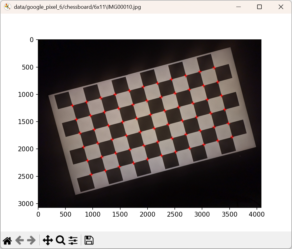
Exercise 5. Modify the program calibration_chessboard.py in order to integrate chessboard detection on images. The function calibrate_chessboard(image_files) has to be modified as follows: Ensure that the program is running fine by checking that each image is displayed with detected corners on it (each corner is represented as a red cross):
|
3.4. Detection refinement
Chessboard detection can be optimized by enabling sub-pixel precision. The refinement of detected corners is performed using the OpenCV function:
cv.cornerSubPix(image, corners, winSize, zeroZone, criteria)This function perform a sub-pixel accurate corner location that is based on the observation that every vector from the center to a point located within a neighborhood of is orthogonal to the image gradient at subject to image and measurement noise. Consider the expression:
$$\epsilon _i = {DI_{p_i}}^T \cdot (q - p_i)$$
where ${DI_{p_i}}$ is an image gradient at one of the points $p_i$ in a neighborhood of $q$. The value of $q$ is to be found so that $\epsilon_i$ is minimized. A system of equations may be set up with $\epsilon_i$ set to zero:
$$\sum _i(DI_{p_i} \cdot {DI_{p_i}}^T) \cdot q - \sum _i(DI_{p_i} \cdot {DI_{p_i}}^T \cdot p_i)$$
where the gradients are summed within a neighborhood ("search window") of $q$. Calling the first gradient term $G$ and the second gradient term $b$ gives:
$$q = G^{-1} \cdot b$$
The algorithm sets the center of the neighborhood window at this new center $q$ and then iterates until the center stays within a set threshold.
The function parameters are:
- image: the input image (grayscaled)
- corners: the detected corners (from cv.findChessboardCorners())
- winSize: Half of the side length of the search window (in pixel). For example, if winSize=(5,5), a $(5*2+1) \times (5*2+1) = 11 \times 11$ search window is used.
- zeroZone: Half of the size of the dead region in the middle of the search zone over which the computation is ignored. The value of (-1,-1) indicates that there is no such a size.
- criteria: Criteria for termination of the iterative process of corner refinement. That is, the process of corner position refinement stops either after criteria.maxCount iterations or when the corner position moves by less than criteria.epsilon on some iteration.
|
Exercise 6. Modify the program calibration_chessboard.py in order to integrate chessboard detection refinement. Within the function calibrate_chessboard(image_files), the existing code: has to be replaced with: Ensure that the program still detect correctly the chessboard. |
3.5. Calibration computation
Camera calibration work with determining the parameters to pass from corners position on an image to a corner position in the 3D worlds. For this purpose, it is needed to express the correspondences between 2D and 3D points. For that, two arrays have to be created, containing for a same index I, the 3D coordinates in one array and the 2D coordinates of the corner in the second array.
|
Exercise 7. Modify the program calibration_chessboard.py in order to integrate chessboard detection refinement. Within The function calibrate_chessboard(image_files), two arrays have to be declared at the beginning : These arrays have to be updated after the corner detection of an image. For that, the code: has to be replaced by: Ensure that the modifications have not broke your code. |
The last information needed to perform the calibration is the size of the input images. This size can be obtained using OpenCV integrated functions.
|
Exercise 8. Modify the program calibration_chessboard.py in order to perform image size retrieval. Within The function calibrate_chessboard(image_files), two variables have to be declared at the beginning of the function: For each loaded image, its size can be obtained by replacing the code: by: Ensure that the program is running without error. |
The pinhole camera model enables to describe the projection of a 3D point $P_{c}\ =\ (x_{c},\ y_{c},\ z_{c})$ onto an image $i$ as a 2D point $(u_{c}^{i},\ v_{c}^{i})$. More formally:
$$\left[{}\begin{array}{c}u_{c}^{i} \\ v_{c}^{i} \\ 1 \end{array}\right]{}\ =\ \left[{}\begin{array}{c} f_{u} & 0 & c_{u} \\ 0 & f_{v} & c_{v} \\ 0 & 0 & 1 \end{array}\right]\ \Delta{}\left({}\left[{}\begin{array}{c} \dfrac{r_{11}^{i}x_{c}\ +\ r_{12}^{i}y_{c}\ +\ r_{13}^{i}z_{c}\ +\ t_{x}^{i}}{r_{31}^{i}x_{c}\ +\ r_{32}^{i}y_{c}\ +\ r_{33}z_{c}\ +\ t_{z}^{i}} \\ \\ \dfrac{r_{21}^{i}x_{c}\ +\ r_{22}^{i}y_{c}\ +\ r_{23}^{i}z_{c}\ +\ t_{x}^{i}}{r_{31}^{i}x_{c}\ +\ r_{32}^{i}y_{c}\ +\ r_{33}z_{c}\ +\ t_{z}^{i}} \\ \\ 1 \end{array}\right]{}\right)$$
where $\Delta{}$ is the distortion computation:
$$\Delta{}\left({} \left[ \begin{array}{c} x_{p} \\ y_{p} \\ \alpha{} \end{array}\right]{}\right){}\ =\ \left[ \begin{array}{c} x_{p} \dfrac{1 + k_1 r^2 + k_2 r^4 + k_3 r^6}{1 + k_4 r^2 + k_5 r^4 + k_6 r^6} + 2 p_1 x_{p} y_{p} + p_2(r^2 + 2 x_{p}^2) + s_1 r^2 + s_2 r^4 \\ \\ y_{p} \dfrac{1 + k_1 r^2 + k_2 r^4 + k_3 r^6}{1 + k_4 r^2 + k_5 r^4 + k_6 r^6} + p_1 (r^2 + 2 y'^2) + 2 p_2 x_{p} y_{p} + s_3 r^2 + s_4 r^4 \\ \\ \alpha{} \end{array}\right],\ r\ =\ x_{p}^{2}+y_{p}^{2}$$
with:
- $f_{u}$, $f_{v}$ respectively are the horizontal and vertical focal lengthes, expressed in pixels
- $c_{u}$, $c_{v}$ are the coordinates of the principal point, expressed in pixels, within the image referential
- $k_{1}$, $k_{2}$, $k_{3}$ are the radial distortion coefficients
- $k_{4}$, $k_{5}$, $k_{6}$ are the radial distortion rational coefficients
- $p_{1}$, $p_{2}$ are the tangential distortion coefficients
- $s_{1}$, $s_{2}$, $s_{3}$, $s_{4}$ are the thin prism distortion coefficients
- $(x_{c},\ y_{c},\ z_{c})$ are the coordinates of the reference point $c$ (i-e the 3D coordinates of the corner $c$)
- $(u_{c}^{i},\ v_{c}^{i})$ are the coordinates of the projection of the reference point $c$ onto the image $i$
- The image $i$ pose is defined such as: $$\left[{} \begin{array}{c} r_{11}^{i} & r_{12}^{i} & r_{13}^{i} & t_{x}^{i} \\ r_{21}^{i} & r_{22}^{i} & r_{23}^{i} & t_{y}^{i} \\ r_{31}^{i} & r_{32}^{i} & r_{33}^{i} & t_{z}^{i} \\ 0 & 0 & 0 & 1 \end{array} \right]$$
By default, OpenCV use a simple radial tangential distortion model where only $k_{1}$, $k_{2}$, $p_{1}$ and $p_{2}$ are computed (all other distortion parameters are set to $0$). In this case, the computation of $\Delta{}$ is:
$$\Delta{}\left({} \left[ \begin{array}{c} x_{p} \\ y_{p} \\ \alpha{} \end{array}\right]{}\right){}\ =\ \left[ \begin{array}{c} x_{p} (1 + k_1 r^2 + k_2 r^4) + 2 p_1 x_{p} y_{p} + p_2(r^2 + 2 x_{p}^2) \\ \\ y_{p} (1 + k_1 r^2 + k_2 r^4) + p_1 (r^2 + 2 y'^2) + 2 p_2 x_{p} y_{p} \\ \\ \alpha{} \end{array}\right],\ r\ =\ x_{p}^{2}+y_{p}^{2}$$
OpenCV enable to compute calibration with the function cv.calibrateCamera. This function determine all the parameters involved within projection equations (including the optical distortion):
ret cv.calibrateCamera(objectPoints, imagePoints, imageSize, cameraMatrix, distCoeffs, rvecs, tvecs, flags = 0)where its parameters are:
- objectPoints: The 3D points (reference points) that compose the calibration reference (the chessboard in our case).
- imagePoints: The 2D projection of the reference points for each image (the refined corners in our case)
- cameraMatrix: a $3\times{}3$ matrix that contains camera intrinsics parameters: $$\left[ \begin{array}{c} f_{u} & 0 & c_{u} \\ 0 & f_{v} & c_{v} \\ 0 & 0 & 1\end{array}\right]$$
- distCoeffs: The coefficient of the distortion model. By default (see flags): $$\left[ \begin{array}{c} k_{1} & k_{2} & p_{1} & p_{2}\end{array}\right]$$
- rvecs: A tuple of $i$ vectors that represent the images pose rotational component (i-e for an image $i$, the values $r_{xx}^{i}$)
- tvecs: A tuple of $i$ vectors that represent the image pose translation $(t_{x}^{i},\ t_{y}^{i},\ t_{z}^{i})$
- flags: Properties and parameters for the calibration process, 0 by default (see OpenCV documentation for further use)
With all these information, camera calibration can be performed.
|
Exercise 9. Modify the program calibration_chessboard.py by modifying the function calibrate_chessboard(image_files) from: to Execute the program and check the camera calibration values. |
4. Calibration result
Once the calibration is computed, the results can be interpreted. For the sake of simplicity and a better software modularity, it is interesting to refactor the original code to separate the calibration computation and the processing of its results.
The first step is to add chessboard size (rows, columns) as parameters of the calibration function and to keep a list of the images that have been used during the calibration process.
|
Exercise 10. Modify the program calibration_chessboard.py by modifying the function calibrate_chessboard(image_files) from: to: The used_image variable has to be updated with all images that are selected during the calibration process by modifying: with: As the function calibrate_chessboard has been modified, the main function has to be updated by replacing: with: Ensure that the modified program is still running. |
The function that compute the calibration has to become an utility function that only make processing and returs results. The results that have been produces has to be returned to the main program.
|
Exercise 11. Modify the program calibration_chessboard.py and add a return instruction to the function calibrate_chessboard in order to return the computed results: The main function has to be modified to retrieve the returned parameters: |
With all results available from the main program, it is possible to modularize the displays. The first step is to externalize the display of the chessboard corners detection from the calibrate_chessboard function.
|
Exercise 12. Modify the program calibration_chessboard.py by adding the function display_detection(image_files, projections) defined such as: This function reuse the display code that was originally within calibrate_chessboard. Now all the display related code present within the function can be deleted by modifying: into: To maintain the display active, the main function has to be updated as follows: Run the program and ensure that the chessboard detection on images is well displayed. |
The calibration function also return the 3D position of the reference points (within the reference_points variable) and the 3D positions of the images (stored within the tvecs variable). It is possible to display all these informations within MatPlotLib.
Before displaying the results, some computations have to be done has OpenCV:
- Give the camera pose as a couple rotation vector (rvec), translation vector (tvec) instead a $4\times{}4$ transform
- The camera pose represent the pass from camera referential to global referential, that is the inverse of the transform we are expecting
Computing the image position from its rvec and tvec values need first to convert the rotatrion vector into a $3\times{}3$ rotation matrix. This can be done using the code:
rotation_matrix = np.eye(3)
cv.Rodrigues(rvec, rotation_matrix)
The first line initialize a $3\times{}3$ matrix and the second line transform the rotation vector into a rotation matrix using Rodrigues transformation.
Once the rotation matrix is obtained, the image position (tvec) has to be inverted according the rotation matrix as OpenCV gives the inverse of the expectedtransform. This can be done using:
position = -rotation_matrix.transpose().dot(tvec)It is now possible to display all the positions.
|
Exercise 13. Modify the program calibration_chessboard.py by adding the function display_positions(reference_points, images_positions, image_rotations) defined such as: This function display within MatPlotLib the reference points (the chessboard corners) as red cross and the image positions as green stars. It is pobbible to activate this display by modifying the main function as follows: Run the program and ensure that the reference points and the cameras positions are well displayed. |
Camera calibration is the preliminary step in visual-based 3D reconstruction. Numerous tools are available for reconstructing scenes or objects in 3D from images, using camera calibration parameters as input data. It is therefore important to be able to save these parameters, for example within a file.
|
Exercise 14. Modify the program calibration_chessboard.py by adding the function export_camera_parameters(camera_matrix, dist_coefs) defined such as: Perform a call to the function export_camera_parameters by modifying the main function as follows: Run the full program and check within the created camera_parameters.txt file the calibration parameters. |
You have now a complete program that can perform a camera calibration.
5. Custom camera calibration
Using the calibration_chessboard.py program, it is possible to calibrate any camera according to a chessboard.
|
Exercise 15. Choose a camera (for example a smartphone) and process to its calibration. For that:
|