This work illustrates the visual 3D reconstruction of a scene according to the Structure from Motion (SfM) method and its implementation within COLMAP software.
1. Structure from Motion
Structure from Motion (SfM) is a photogrammetric approach that enables to produce a 3D model (Structure) of an inert scene from multiple images of it (Motion). This approach involves solving the projection equations system that links the camera parameters (calibration), the positions of the scene's points on the images and the 3D positions of these points within the scene. More formally:
$$\begin{cases}u_{i}\ =\ \dfrac{f_{u}r_{11}x_{t}\ +\ f_{u}r_{12}y_{t}\ +\ f_{u}r_{13}z_{t}\ +\ f_{u}t_{x}}{r_{31}x_{t}\ +\ r_{32}y_{t}\ +\ r_{33}z_{t}\ +\ t_{z}}\ +\ c_{u} \\ \\ v_{i}\ =\ \dfrac{f_{v}r_{21}x_{t}\ +\ f_{v}r_{22}y_{t}\ +\ f_{v}r_{23}z_{t}\ +\ f_{v}t_{x}}{r_{31}x_{t}\ +\ r_{32}y_{t}\ +\ r_{33}z_{t}\ +\ t_{z}}\ +\ c_{v} \end{cases}$$
where:
- $(u_{i},\ v_{i})$ is the 2D projection of the point $(x_{t},\ y_{t},\ z_{t})$ ont the image $i$
- $f_{u},\ f_{v},\ c_{u}, c_{v}$ are the camera intrinsic parameters
- The camera pose for the production of image $i$ is: $\begin{bmatrix}r_{11} & r_{12} & r_{13} & t_{x} \\ r_{21} & r_{22} & r_{23} & t_{y} \\ r_{31} & r_{32} & r_{33} & t_{z} \\ 0 & 0 & 0 & 1 \end{bmatrix}$
With enough 3D points, images and 2D projections, the produced linear system can be solved and enables to retrieve all the involved variables.
2. COLMAP
COLMAP is a visual 3D reconstruction software that relies on Structure From Motion (SfM) photogrammetric approach. This software aims to produce photogrammetric 3D models from a set of images from calibrated cameras. The software is fully installed and functionnal onto the room's computer. However, for those wishing to work on their own computers, COLMAP can be installed on multiple architectures / systems by following the installation documentation.
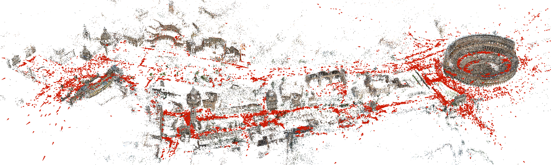 Sparse model of central Rome using 21K photos produced by COLMAP’s SfM pipeline (c) COLMAP
COLMAP's SfM process is designed to be efficient and to handle a large number of points automatically. To achieve this, several constraints are necessary:
- All the involved images have to come from calibrated cameras ($f_{u},\ f_{v},\ c_{u}, c_{v}$ camera parameters and distortion have to be known)
- The 3D points are automatically selected using Feature Detection methods (they cannot be fixed by user)
Producing a 3D reconstruction with COLMAP use the following process:
- Camera Calibration (using OpenCV for example)
- Image shooting of the scene
- Feature Detection on the images
- Solving SfM
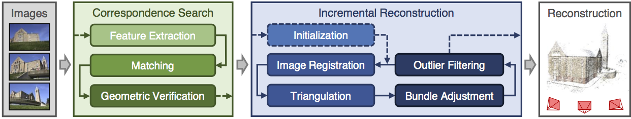 COLMAP SfM Pipeline (c) COLMAP
2.1. First steps
To discover how COLMAP works, we're going to work on a dataset containing images and calibration information.
|
Exercise 1. Create a cv-pw-colmap folder on a local disk on your computer. Warning: (be carefull to not create the folder on shared / cloud folders as COLMAP intensively uses the filesystem when running) Download the south-building example data and unzip the file within the cv-pw-colmap folder On linux systems:
On windows systems:
COLMAP project directory follows standard structure and are made of:
Check that the downloaded folder is well structured. Expected structure is: cv-pw-colmap |
COLMAP provides a Graphical User Interface (GUI) for processing projects. This interface enable to have a visual control on the process. All of the tasks that enable to process a dataset can be achieved from the GUI.
|
Exercise 2. Launch the COLMAP GUI: on Linux systems: colmap gui on Windows systems: run COLMAP.bat program Ensure that the GUI is displaying and is reactive. |
2.2. Project setup
The processing of a Structure from Motion within COLMAP is called a project. From the downloaded data, a project has to be set up before starting the 3D reconstruction.
|
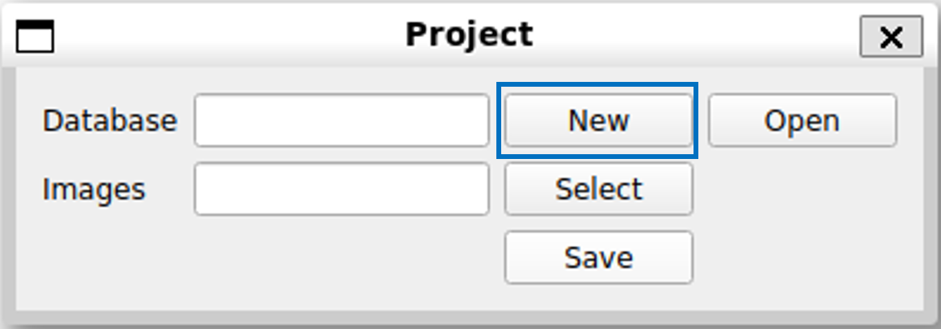
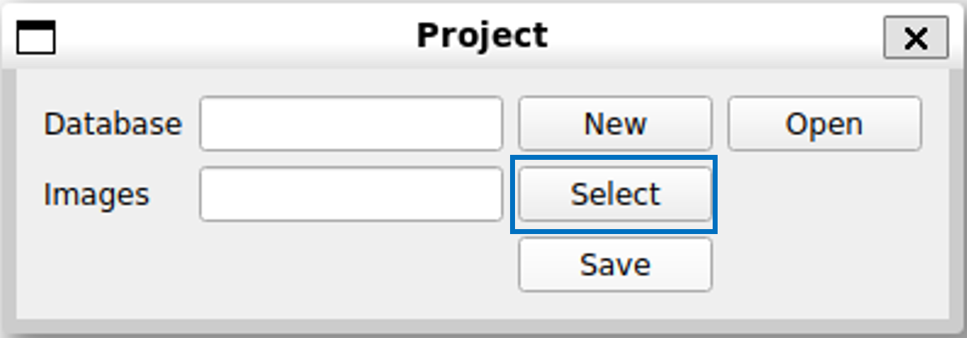
Exercise 3. COLMAP use an embedded relationnal database to store all the 3D reconstruction related information. When a new project is started, a new database has to be set up. Within the COLMAP GUI, within the menu File, click on the New Project item. Within the new Project window, click on the New button at the right of the Database field
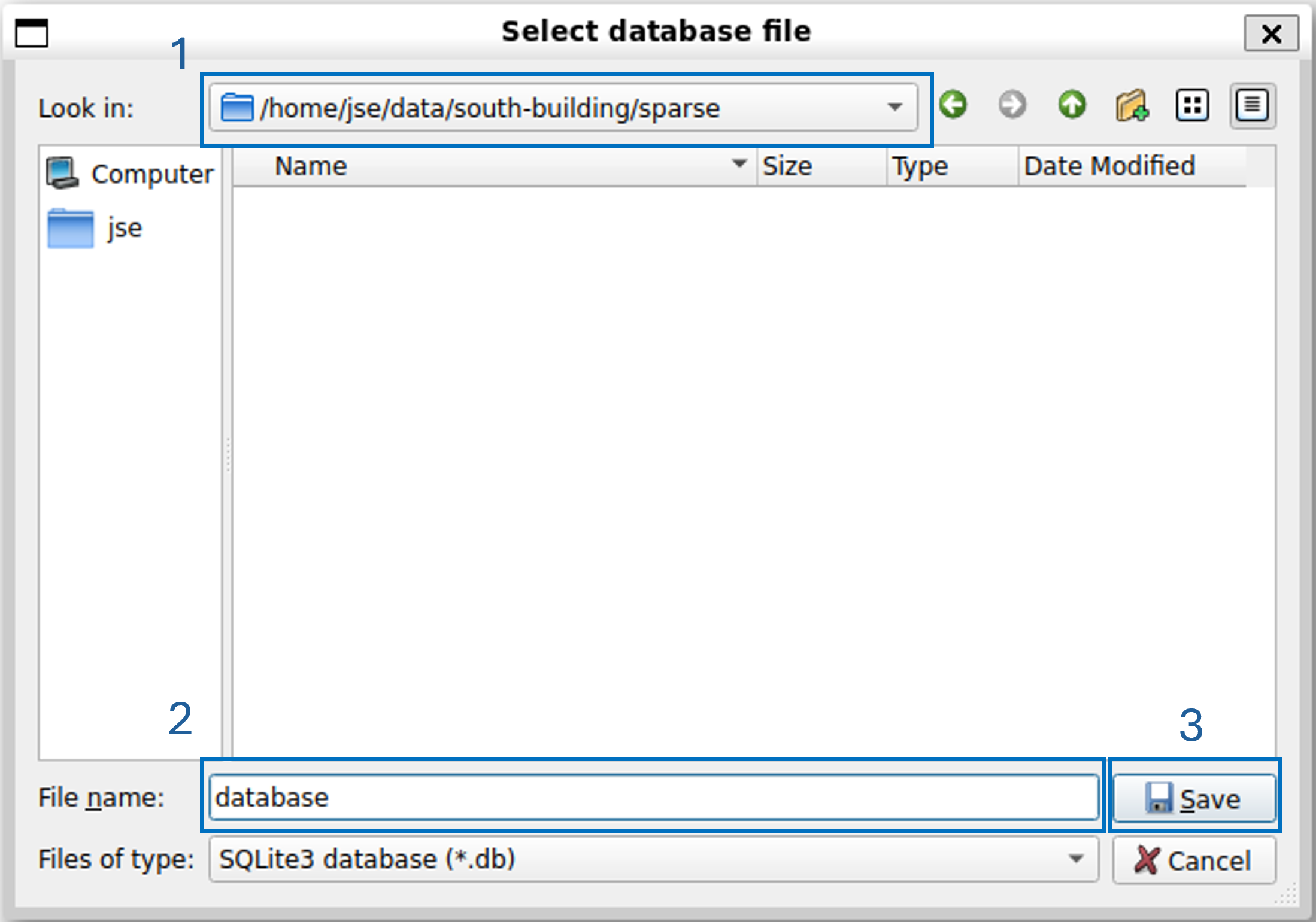
Within the Select database window:
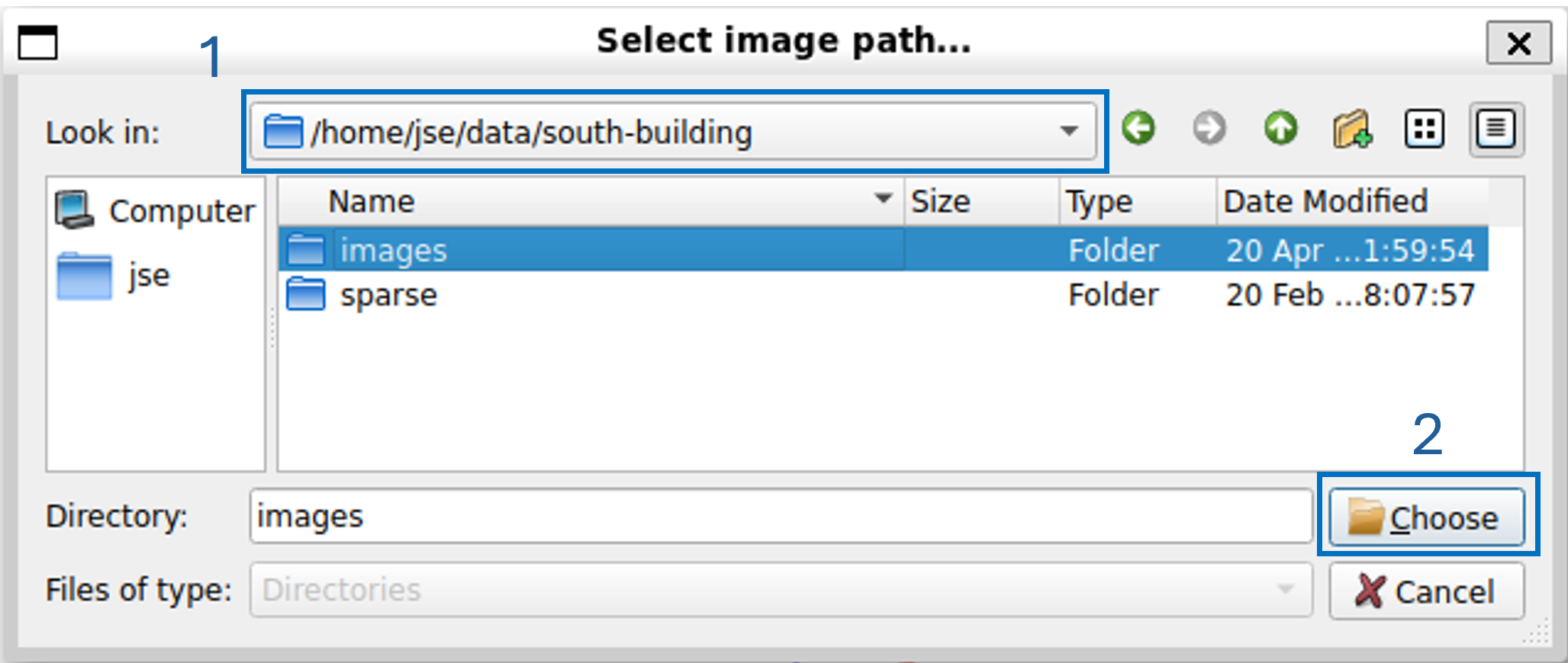
The location of the project images has now to be set up. Back to the Project window, click on the Select button at the right of the Images field
Within the new Select images path... window:
Back within the Project window, click on the Save button |
2.3. Camera model
COLMAP process relies on calibrated cameras (i-e cameras for which intrinsics parameters, uncluding distortion parameters, have previously been computed). As there is various means and various libraries or software that enables to calibrate cameras, COLMAP can deal with differents formats. These formats are determining the parameters that appears within the sparse/cameras.txt file. The available camera models are:
| COLMAP type | Description | Parameters (cameras.txt) | Note |
| SIMPLE_PINHOLE | Pinhole camera with square pixels and no distortion | $f\ c_{x}\ c_{y}$ | For undistorted input images. |
| PINHOLE | Pinhole camera with possible non square pixels | $f_{x}\ f_{y}\ c_{x}\ c_{y}$ | |
| SIMPLE_RADIAL | Pinhole camera with square pixels and simple radial distortion | $f\ c_{x}\ c_{y}\ k$ | Camera model of choice, if the intrinsics are unknown and every image has a different camera calibration, e.g., in the case of Internet photos. |
| SIMPLE_RADIAL_FISHEYE | Fisheye camera with square pixels and simple radial distortion | $f\ c_{x}\ c_{y}\ k$ | |
| RADIAL | Pinhole camera with square pixels and two parameters radial distortion | $f\ c_{x}\ c_{y}\ k_{1}\ k_{2}$ | |
| RADIAL_FISHEYE | Fisheye camera with square pixels and two parameters radial distortion | $f\ c_{x}\ c_{y}\ k_{1}\ k_{2}$ | |
| OPENCV | Pinhole camera calibration from OpenCV with default parameters | $f_{x}\ f_{y}\ c_{x}\ c_{y}\ k_{1}\ k_{2}\ p_{1}\ p_{2}$ | For cameras that have been calibrated using OpenCV (see Camera Calibration practical work) |
| OPENCV_FISHEYE | Fisheye camera calibration from OpenCV with default parameters | $f_{x}\ f_{y}\ c_{x}\ c_{y}\ k_{1}\ k_{2}\ p_{1}\ p_{2}$ | |
| FULL_OPENCV | Pinhole camera calibration from OpenCV with rationnal radial distortion parameters | $f_{x}\ f_{y}\ c_{x}\ c_{y}\ k_{1}\ k_{2}\ p_{1}\ p_{2}\ k_{3}\ k_{4}\ k_{5}\ k_{6}$ | |
| FOV | Field Of View (FOV) camera | $f_{x}\ f_{y}\ c_{x}\ c_{y}\ \omega$ | Model from Google Project Tango (discontinued, replaced by ARCore). Make sure to not initialize $\omega$ to zero) |
| THIN_PRISM_FISHEYE | Pinhole camera with radial, tangential and thin prism distortion | $f_{x}\ f_{y}\ c_{x}\ c_{y}\ k_{1}\ k_{2}\ p_{1}\ p_{2}\ k_{3}\ k_{4}\ sx_{1}\ sy_{1}$ | |
| RAD_TAN_THIN_PRISM_FISHEYE | Fisheye camera with radial, tangential and thin prism distortion | $f_{x}\ f_{y}\ c_{x}\ c_{y}\ k_{0}\ k_{1}\ k_{2}\ k_{3}\ k_{4}\ k_{5}\ p_{0}\ p_{1}\ s_{0}\ s_{1}\ s_{2}\ s_{3}$ |
2.4. Processing
The 3D reconstruction of a scene is a multi-step process that can be split into feature detection and matching (detecting the 2D positions of the 3D points projection within the images) and the SfM solving for retrieving 3D points position and camera poses.
2.4.1. Feature Matching
Feature matching enables to detect the most interesting 3D points for the reconstrction. A point is considered a point of interest if it is easy to spot, even on images at different scales and with different rotations, and if it is seen on a significant number of images. COLMAP uses the SIFT (Scale Invariant Feature Transform) algorithm to detect and match points of interest within images. In practice, the points detected by SIFT are those with a high contrast to their surroundings.
With COLMAP, the detection and matching of points of interest is carried out in two stages:
- Detection of potential points of interest (Feature Extraction)
- Matching detected points between images (Feature Matching)
|
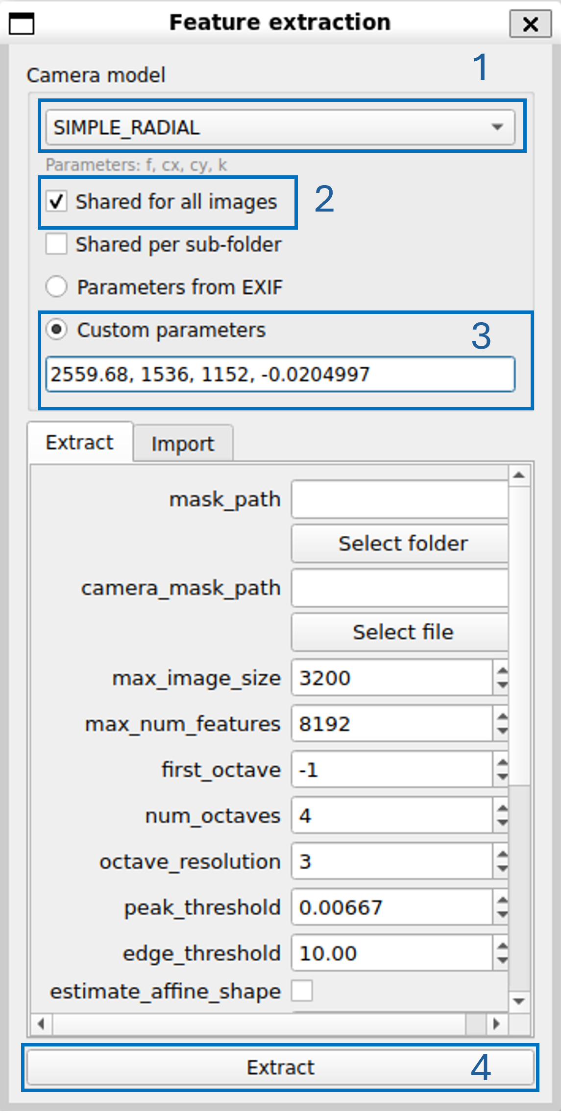
Exercise 4. Within the COLMAP window, from the Processing menu, select the Feature Extraction item. Within the new Feature Extraction window:
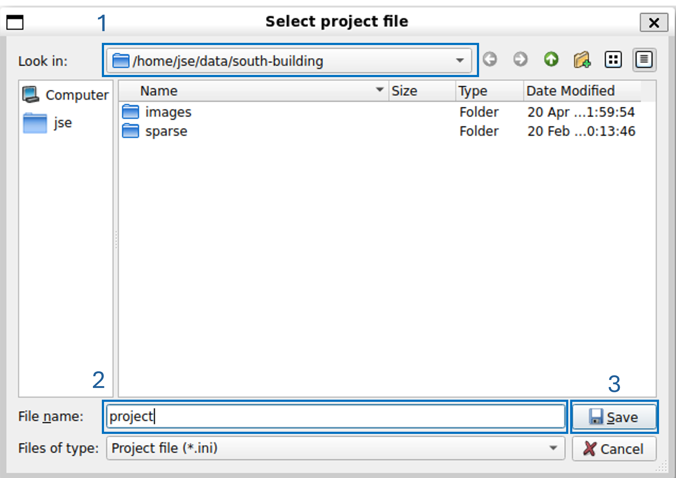
The extraction is performed (a progress windows appears). At the end of the process, the Feature Extraction windows can be closed. Back to the main window, save the project by opening menu File then clicking on Save project item. Within the Select project file window:
|
Potential points of interest are now detected. All the parameters of the Feature extraction window are related to SIFT implementation. The complete description of these parameter can be found within the SIFT publication. The next step is to match the potential points of interest in order to construct a set of 3D points projection.
|
Exercise 5. Within the COLMAP window, from the Processing menu, select the Feature Matching item. Within the new Feature matching window, click on the Run button. The parameters that are available within the Feature matching windows are related to SIFT matching algorithm and should not be modified. For more information, check the SIFT publication. Once the process is finished, the Feature matching window can be closed. |
When the feature matching is done, the 3D reconstruction can be computed.
2.4.2. Sparse 3D reconstruction
3D reconstruction consists of two complementary phases. The first builds the photogrammetric model (camera poses and 3D positions of points of interest) in an approximate way, by incrementally adding the images one by one and calculating their positions in relation to each other. This is called the relative orientation phase.
Once relative orientation has been completed for all images, the poses and 3D positions of points of interest are refined by bundle adjustment. This is a global refining of the 3D coordinates, the parameters of the poses, and the camera(s) intrinsics parameters. Given a set of images depicting a number of 3D points from different viewpoints. Its name refers to the geometrical bundles of light rays originating from each 3D feature and converging on each camera's optical center, which are adjusted optimally according to an optimality criterion involving the corresponding image projections of all points.
The two phases of relative orientation and bundle adjustment are used to solve the system of equations constructed from the points of interest and their projections.
|
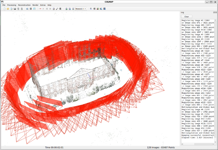
Exercise 6. Within the COLMAP window, from the Reconstruction menu, select the Start reconstruction item. The reconstruction process will start and the GUI will show the incremental relative orientation of the images. Within the GUI, the camera poses are represented in red, the 3D scene is represented in true color.
At the end of the process, project file can be saved by opening the menu File and by selecting the Save project item. |
The resulting reconstruction makes up the photogrammetric model, in which the exposures of each image (as rigid body transformations) and the 3D points have been calculated. However, this low-resolution reconstruction can be further improved.
2.4.3. Image undistort
After the Sfm computation, all parameters that are involved within projection equations are known. A first available post processing is to undistort the input images in order to produce images that are not affected by optical distortion.
|
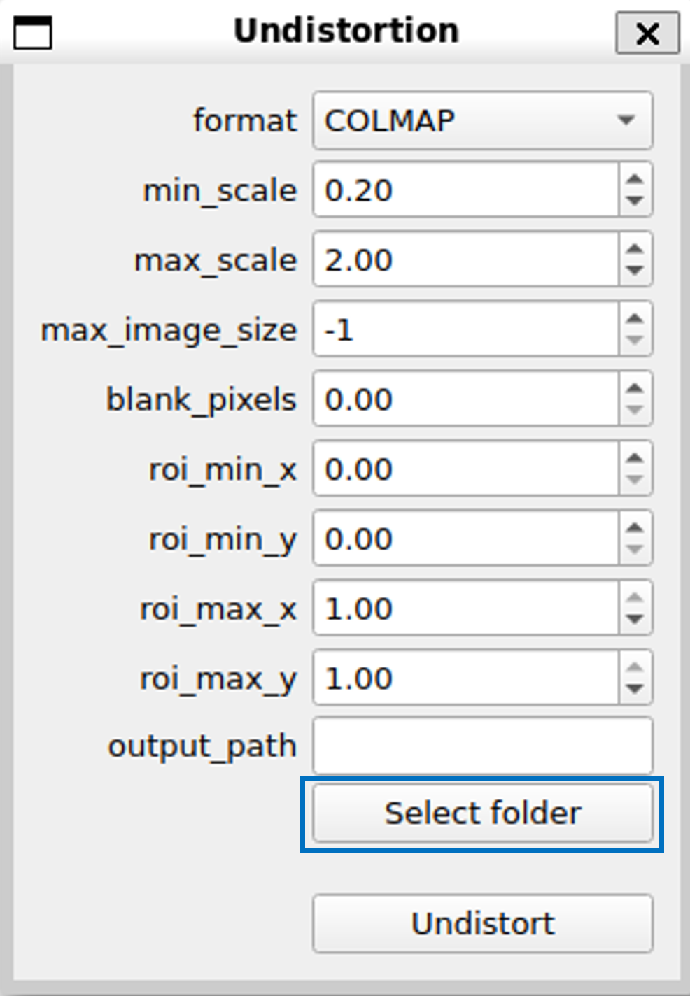
Exercise 7. Within the project directory south-building, create an undistort subdirectory: mkdir south-building/undistort Within the COLMAP GUI, from the menu Extras, select the Undistortion item. Within the new Undistortion windows, click on the Select folder button.
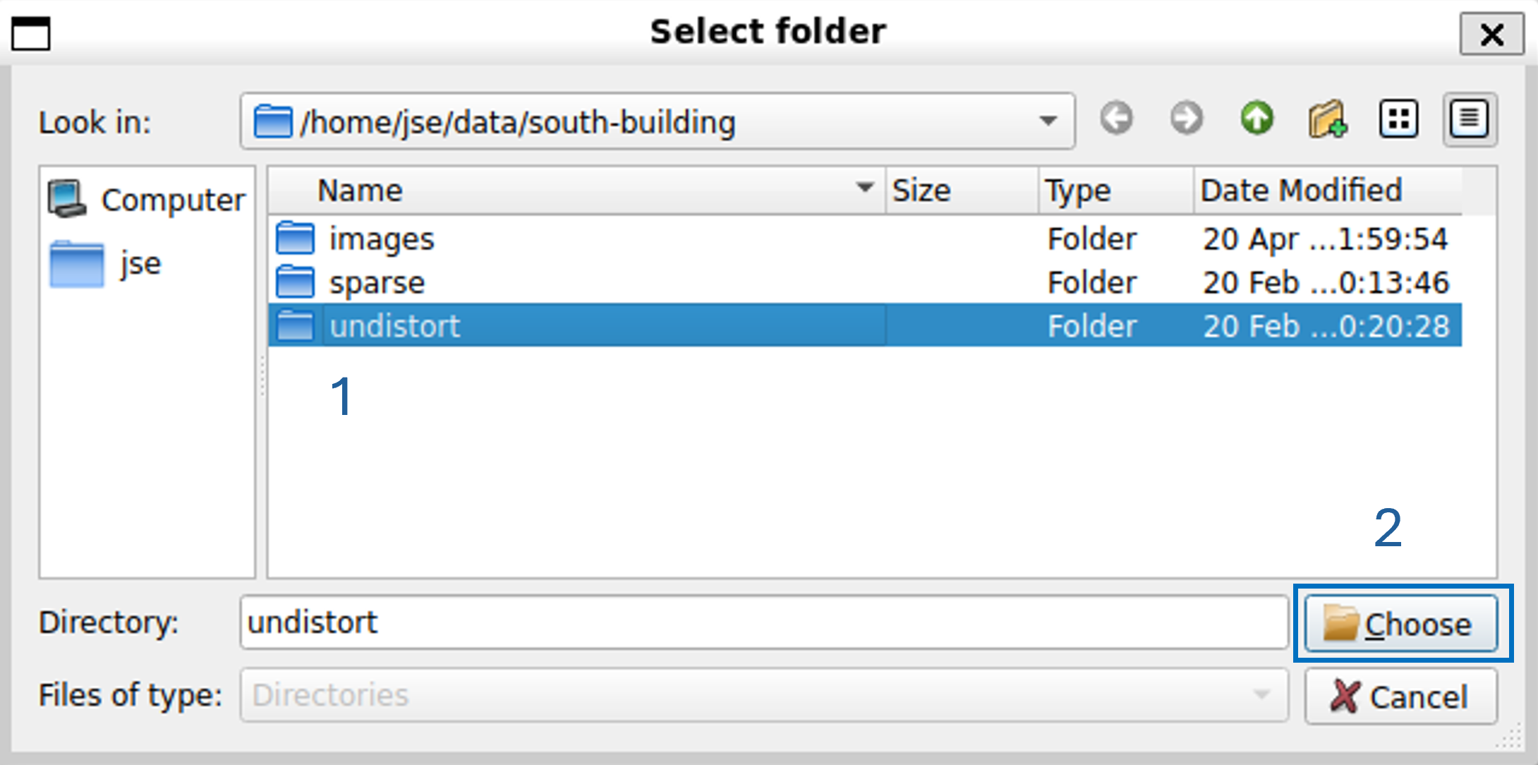
Within the new Select folder window:
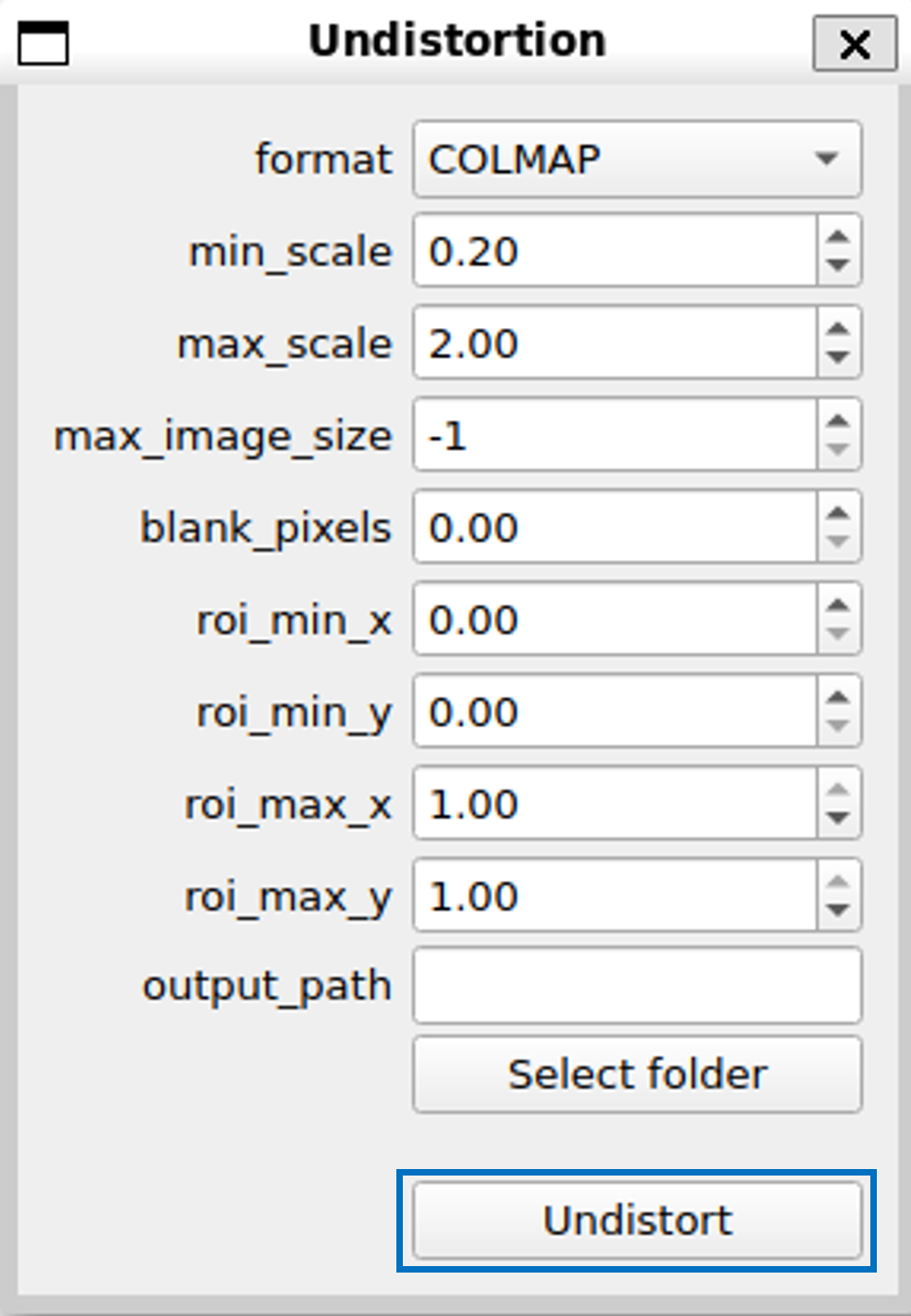
Back to the Undistortion windows, click on the Undistort button.
The undistortion of the images is processed. At the end, the south-building/undistort subdirectory contains undistorted images. The Undistortion window can be closed and the project can be saved by opening the menu File and by selecting the Save project item. |
3. Visualization
Once the COLMAP part of the process has been completed, the tools used no longer offer an integrated visualization of the results. In order to always be able to visualize the models produced, it is necessary to use visualization software such as MeshLab. that is an open source system for processing and editing 3D triangular meshes.
It provides a set of tools for editing, cleaning, healing, inspecting, rendering, texturing and converting meshes. It offers features for processing raw data produced by 3D digitization tools/devices and for preparing models for 3D printing.
|
Prerequisite If MeshLab is not available on the system, it can be installed from its website. On windows systems
On linux systems
Once MeshLab is installed, try to run the program. |
MeshLab will be used as the visualization software for the next part of this works.
4. Dense surface reconstruction
The dense surface reconstruction is the final step of the global 3D reconstruction process. It is dedicated to the production of a photoralistic topological 3D model from the SfM computation. Even if COLMAP can handle a part of this process, its computing performance are too limited to produce a result within an acceptable time. The use of another tool is required.
OpenMVS (Open MultiView Stereo) is a library for computer-vision scientists and especially targeted to the Multi-View Stereo reconstruction community. While there are mature and complete open-source projects targeting Structure-from-Motion pipelines (like COLMAP, OpenMVG, ...) which recover camera poses and a sparse 3D point-cloud from an input set of images, there are none addressing the last part of the photogrammetry chain-flow. OpenMVS aims at filling that gap by providing a complete set of algorithms to recover the full surface of the scene to be reconstructed. The input is a set of camera poses plus the sparse point-cloud and the output is a textured mesh. The main topics covered by this project are:
- dense point-cloud reconstruction for obtaining a complete and accurate as possible point-cloud
- mesh reconstruction for estimating a mesh surface that explains the best the input point-cloud
- mesh refinement for recovering all fine details
- mesh texturing for computing a sharp and accurate texture to color the mesh
OpenMVS binaries are available for windows and linux.
|
Prerequisite OpenMVS can be installed by inflating the binary archive that correspond to your system. If OpenMVS is not available on the system, it can be installed from its GITHUB repository. On windows systems
On Linux system
|
4.1. Dense reconstruction
OpenMVS can be used after COLMAP processing for enhancing results. The first step that can have to be processed is the construction of a dense points cloud reconstruction. It is possible to densify the model by ensuring that as many image pixels as possible can produce a 3D point. OpenMVS dense reconstruction relies on the Accurate Dense and Robust MultiView Stereoposis (MVS) algorithm and its optimization Clustering Views for Multi-view stereo (CMVS).
This step will produce a lot of new points from the sparse model produced by COLMAP. The dense reconstruction need the images poses and the undistorted raster that have been computed with COLMAP. The OpenMVS is mostly a library and has to be used from a command line.
|
Exercise 8. The first step is to prepare the data coming froml COLMAP to be integrated to OpenMVS. For that:
InterfaceCOLMAP -i undistort -o dense/scene.mvs --image-folder undistort/images After the command, the folder should be structured as follows: cv-pw-colmap |
Now all the needed data are available, the dense reconstruction can be processed from scene.mvs. The dense reconstruction algorithm first computes the DethMaps that correspond to input images. A depth map is an image of the same size as the original image, but for which each pixel represents a depth (the distance from the point represented by that pixel along the camera's $Z$ axis).
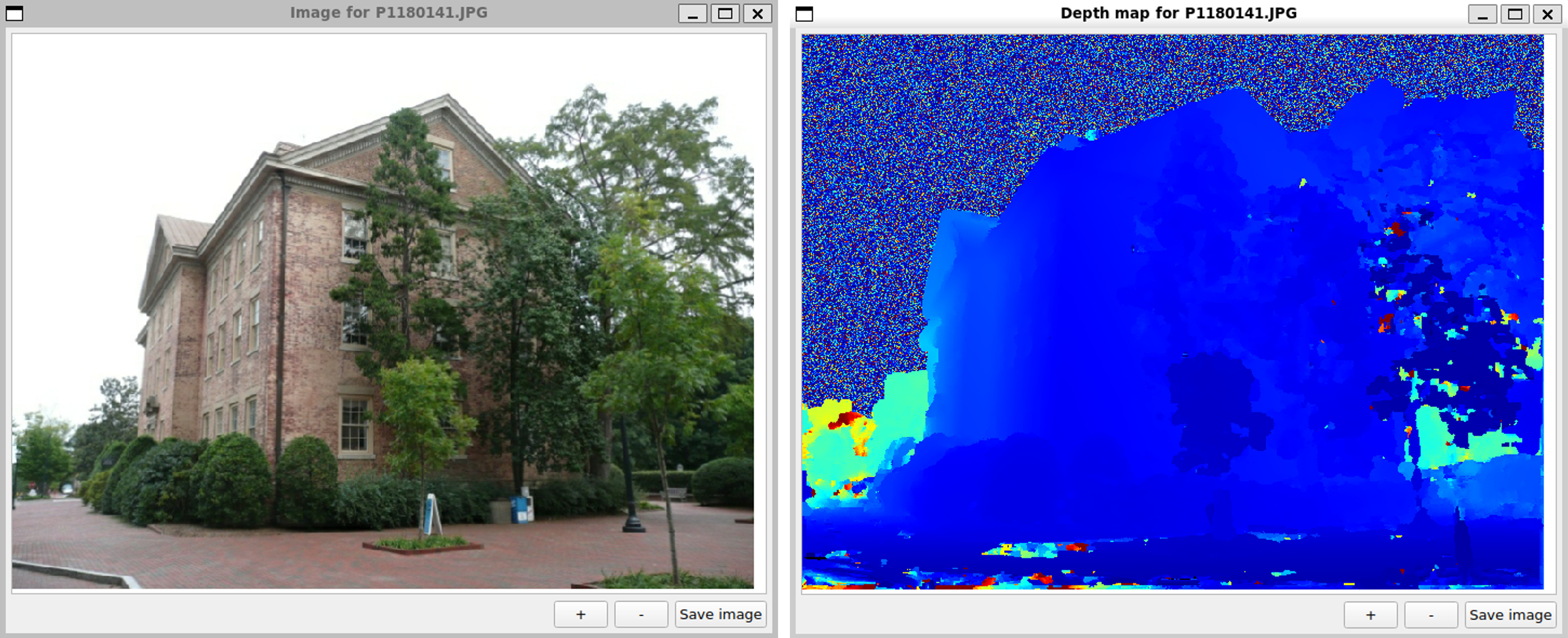
Once the depth maps are computed, the algorithm merges them and computes pixels 3D position according to their depths. Each pixel with a determinated depth can produce a 3D point.
|
Exercise 9. From a terminal:
DensifyPointCloud scene.mvs The densification algorithm is running anf after few minutes the result is available as a scene_dense.ply file. Note that all the computed deapth maps are present as .dmap files within the dense folder. The dense_scene.ply file can be opened with MeshLab:
|
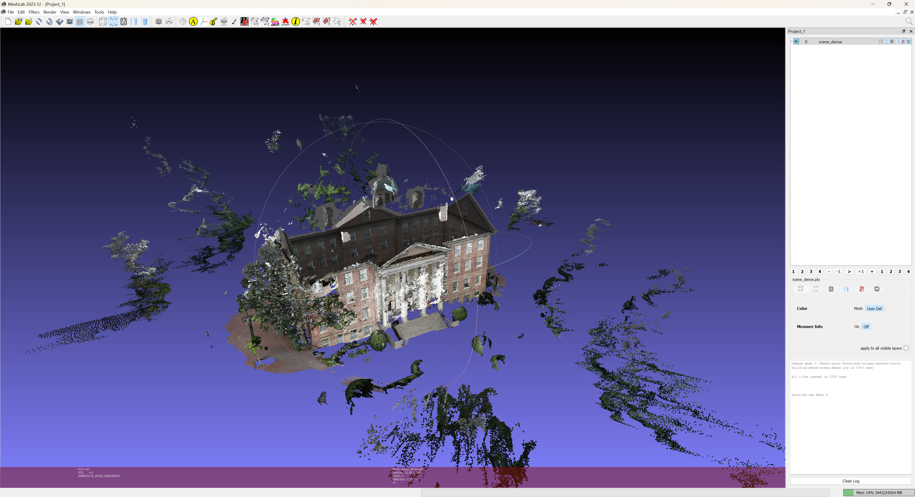
The densification produce a lot of points but also add some noise (bad points). The noise can be ignored as this time. it is now possible to reconstruct a surface by meshing the points.
4.2. Surface reconstruction
Although the dense point cloud has a resolution that gives the visual impression that the model is a continuous surface, zooming in on it reveals that this is not the case. Reconstructing a surface from the point cloud adds topological information to the 3D model by linking points with edges and faces, known as meshes.
|
Exercise 11. From a terminal:
ReconstructMesh scene_dense.mvs -p scene_dense.ply The software will produces (within few minutes) a scene_dense_mesh.ply file that contains the 3D surface reconstructed from 3D dense points. It is possible to view scene_dense_mesh.ply using MeshLab:
|
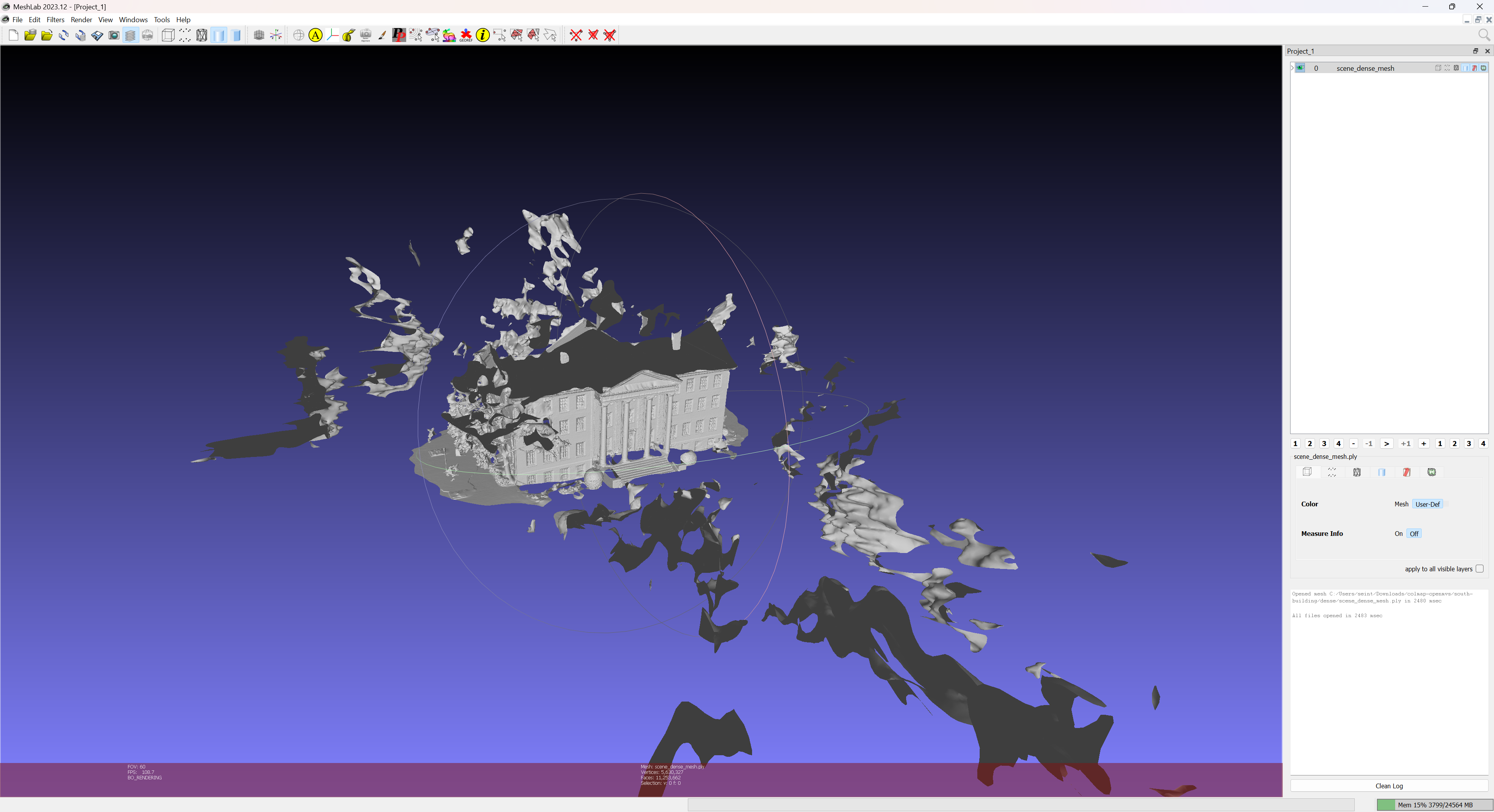
The surface still contains some noise (to be dealt with later) and has a few imperfections that can be corrected by surface refinement.
|
Exercise 12. [OPTIONAL] Warning: Mesh refinement can take a long time (on the order of one or even several hours). It is recommended to perform this step only on high capacity computers. From a terminal:
RefineMesh scene_dense.mvs -m scene_dense_mesh.ply -o scene_dense_mesh_refine.mvs --scales 1 --max-face-area 16 The input dense mesh will be refined and dorrected and the result is saved within the scene_dense_mesh_refine.ply file, that can be visualizated within MeshLab:
|
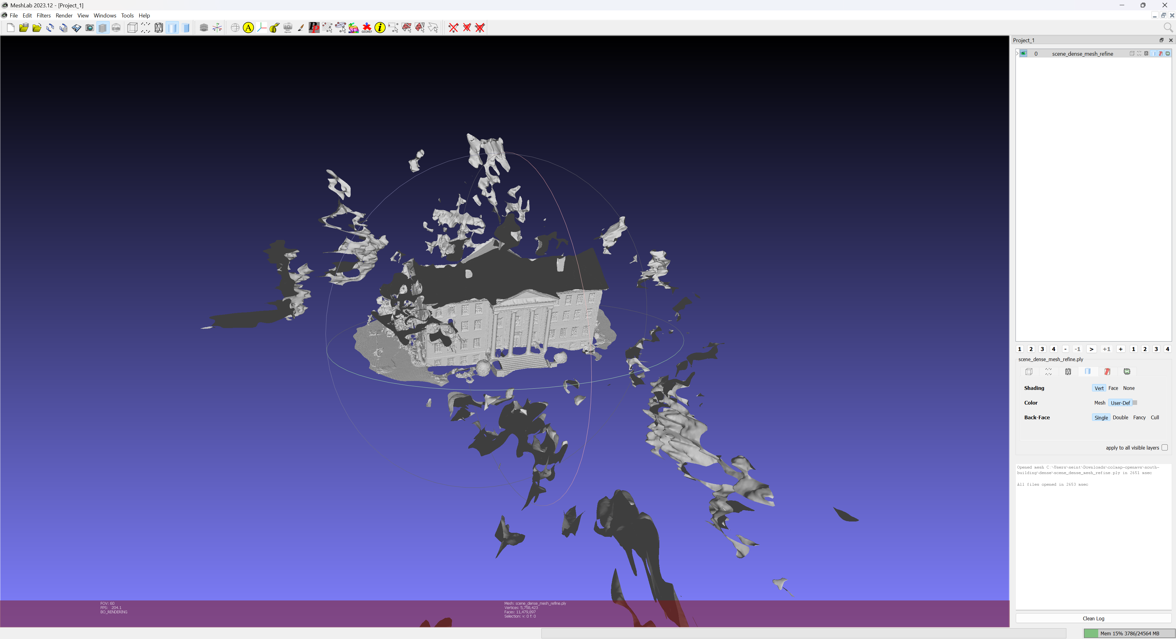
The next step within 3D reconstruction pipeline is to make the 3D mesh photorealistic.
4.3. Texturing
As the mesh is obtained from 3D points that are seen on images (SfM computation), each of its face is linked to a set of images. It is then possible to texture the model using the original input images. The production of a textured mesh is an heavy process that have to compute for each face of the mesh its projection on the available images. Such a computation can take a lot of time and can be parametrized in order to keep an acceptable running time. Available parameters are:
- The decimation factor of the final mesh is the ratio of original faces that are kept within the resulting mesh. This parameter can be usefull for producing meshes with less faces, enabling them to be integrated within 3D visualization software
- The resolution level of the images that indicates a limit resolution for the texture and that enable to avoid the result to need a lot of video memory for displaying.
|
Exercise 13. From a terminal:
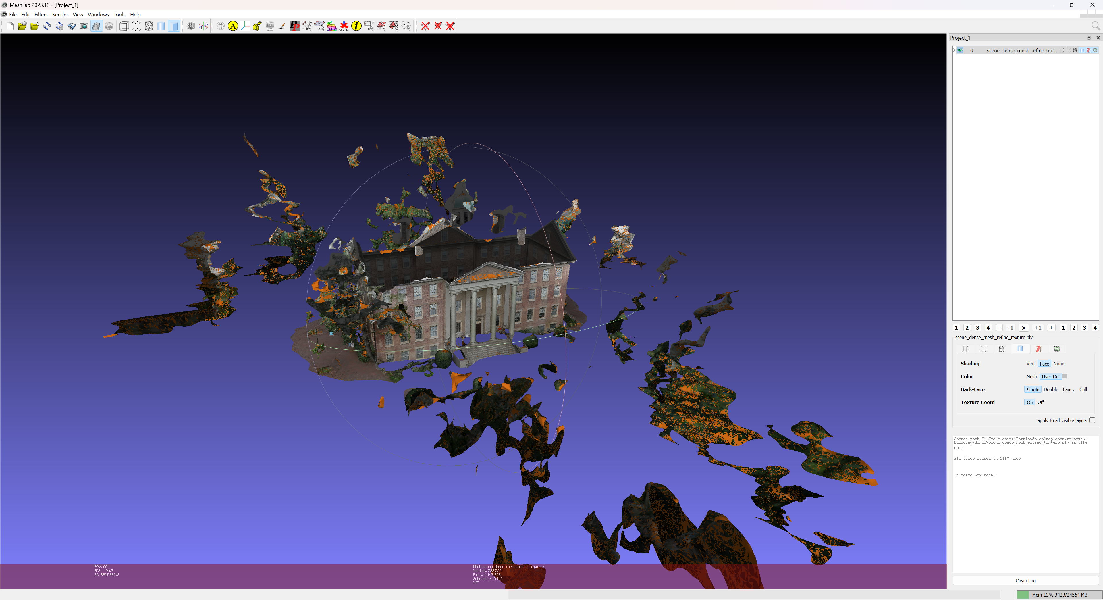
TextureMesh --decimate=0.1 --resolution-level=2 scene_dense.mvs -m scene_dense_mesh_refine.ply -o scene_dense_mesh_refine_texture.mvs Tip: If the refined mesh has not be cmputed (dur to computation limitations), it is possible to replace the scene_dense_mesh_refine.ply input by scene_dense_mesh.ply. The software produces a file scene_dense_mesh_refine_texture.ply that contains a textured mesh that can be opened within MeshLab:
If the system has enough computation capabilities, it is possible to increment the decimate parameter to a value that is near to 1.0. |
The final model is photorealistic but still contains a lot of noise. A model cleaning is necessary.
4. Cleaning and post-processing
To clean a reconstructed model is important before finilyzing the process. This step can be performed manually using the MeshLab software.